Figure 1
Contents
For this project, I set out on a personal endeavor to create a dog breed classifier (133 breeds) with an accuracy at or above 90% using Python. Throughout this project, I explored various models and model structures, beginning with ResNet-18 and ending with a cocktail of concatenated convolutional neural networks (CCCNN). The initial exploratory stages (sections 1-3) were imperative for my personal growth, although, less interesting. So I’ve condensed the first three sections to quickly jump to section 4. Please, stick around until my favorite section, “Jessie and Friends.”
Check out the full GitHub repository here.
A special thanks to Udacity for providing the dataset. The dataset can be found here
Some of the images were either corrupted or not in the standard .jpeg/.png format. In this section we’ll be deleting those files from our dataset.
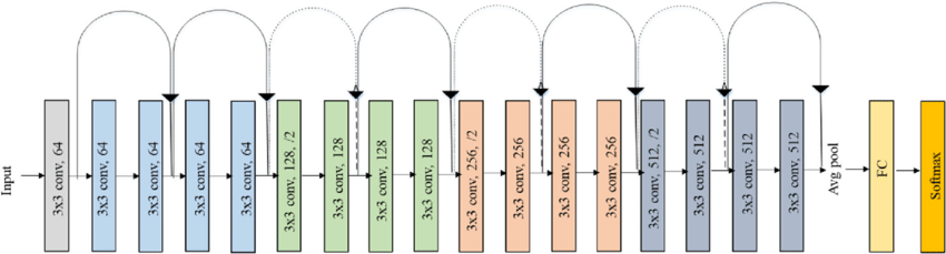
There are a few variations of ResNet, but all of them utilize what's called a "skip connection." In theory, deeper networks should outperform shallower networks, however, in practice, deeper networks suffer from "vanishing gradients," resulting in poorer results. Even if a neural network were to arrive at the theoretical global minium at layer 50 (e.g. out of a 100 layers), it would have trouble maintaining those weights due to the difficulty of learning the identity function. By using skip connections, the neural network is able to better maintain its optimal weights without the identity function. In short, skip connections enable deep neural networks to perform as intended.
In this section, we'll be building ResNet-18 from scratch using the architecture in figure 1.
"image_dataset_from_directory" is a convenient way of loading in your dataset. It loads and labels the dataset depending on its parent directory.
Here, we'll extract the labels.
makes the script below scrollable
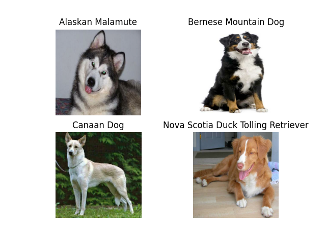
Let's take a look at some of the good doges.
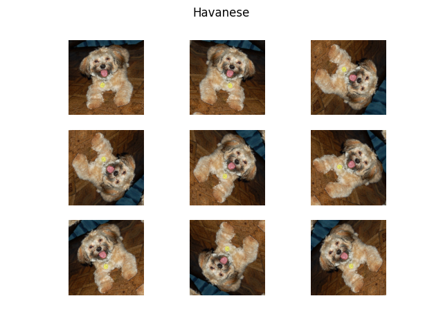
Data augmentation allows us to "create" more datasets by randomly augmenting the images. Here we'll be making a sequential layer that randomly rotates and flips the images. This layer will be embedded into the beginning of the model.
Let's take a look at what this function does.
I had initially set the dropout rate to 0.2, but to adjust for the high variance, I set the dropout rate to 0.5. With this change, there was a significant improvement in variance and a slight improvement in accuracy. Let's take a look at what I'm talking about, but with graphs!
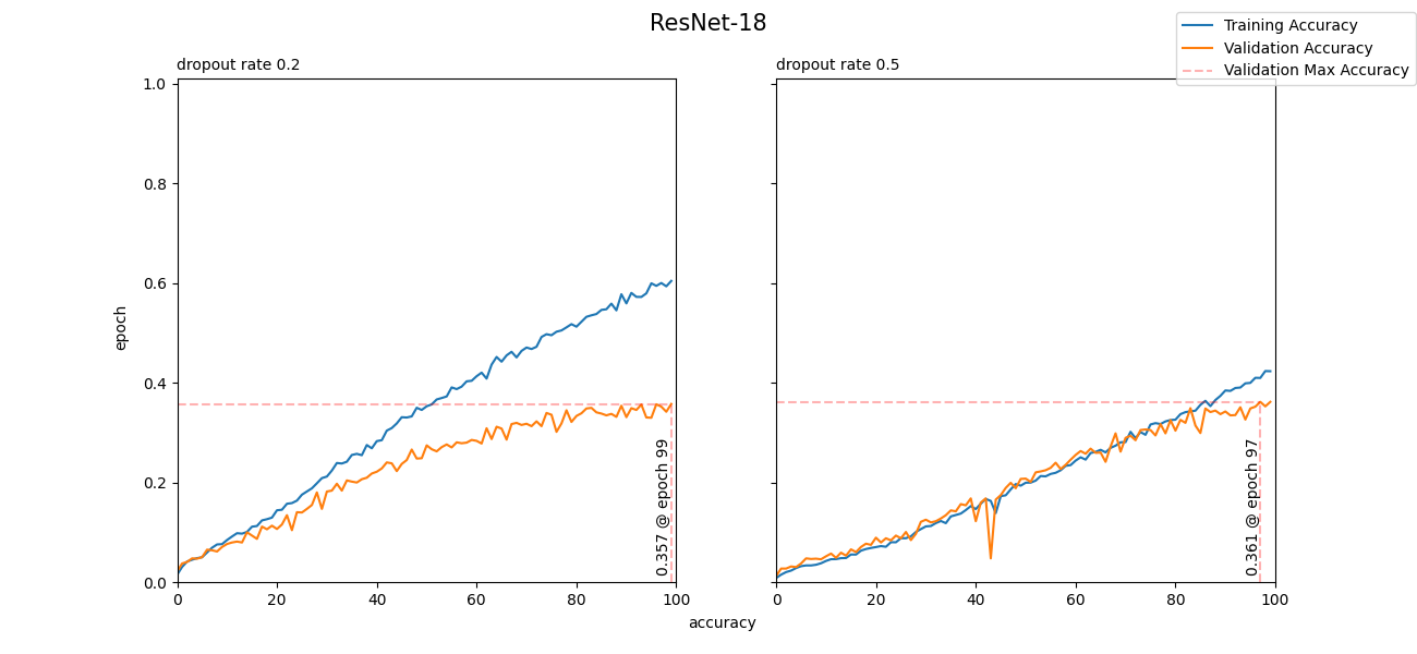
As you can see from figure 4, by increasing the dropout rate, variance significantly decreased with a slight improvement in accuracy. Admittedly, the overall accuracy isn't very impressive, but I wasn't expecting drastic results from ResNet-18, as there are 133 classes. This section was more of a proof of concept and less about results. That isn't to say that ResNet-18 is a bad model. It's a great model for classification problems with less classes. Now, let's move onto something more suitable for this problem, ResNet-50!
In this section, we'll be building ResNet-50 using transfer learning, adding a few more tunable hyperparameters, and exploring models with varying depths.
The first, basic model has three added dense layers (512, 256, 256) and the deeper model has four added dense layers with 512 nodes each. Similar to the function above, we're able to tune the dropout rate with "drop." However, this time, data augmentation is no longer a parameter and is a permanent part of the function. Three additional parameters are "tune_at," "tuning" and "reg." With the parameter "tune_at" we can choose which layer to tune from if "tuning" is set to true. With the parameter "reg," we can adjust the lambda of L2 regularization in the dense layers. Let's get to training!
I had spent a tremendous amount of time attempting to tune ResNet-50. For brevity, I'll display the results of the 3 best models:
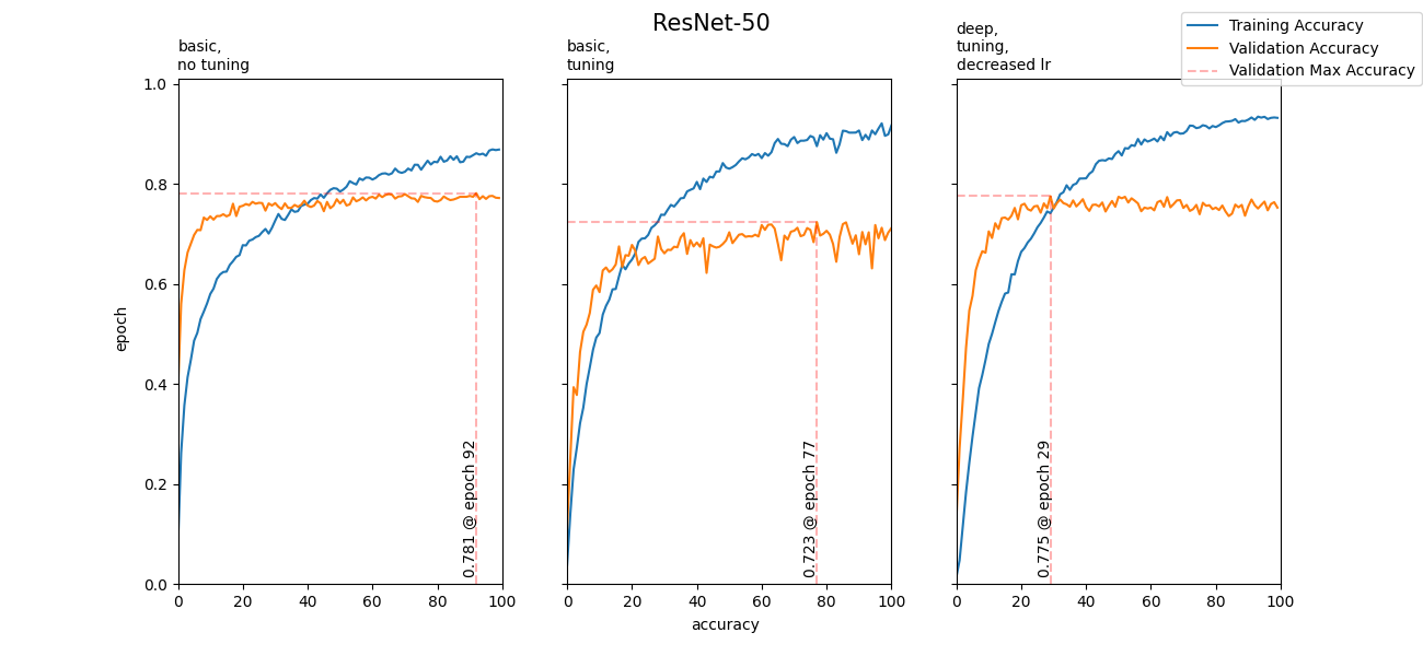
The results definitely were a huge improvement from ResNet-18, however, due to the time it took to run a 100 epochs, it made fine-tuning impractical. In search for a better solution, I discovered bottleneck features and tf.keras.layers.Concatenate(). Prepare for magic.
Before delving into the cocktail of concatenated convolutional neural networks (CCCNN), let's first explore the power of utilizing bottleneck features, separately. Extracting and using bottleneck features is an incredibly efficient way to train your neural network.
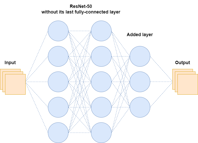
Let's consider a scenario where we've imported ResNet-50 but have replaced its last fully-connected layer with our own. Let's also say we're only interested in training our added layer and have frozen the other layers. During training, the aforementioned model (figure 6) would pass the inputs through all the layers (forward propagation), compute the gradient only for the last added layer (backpropagation) and update the last layer's weights. Since we're only updating the last added layer, the layers before will alway produce the same outcome. In other words, the model is repeatedly making the same computations and passing the same values to the added layer. Mind you, ResNet-50 has a total of 23,587, 712 parameters without it's last fully-connected layer. That's a lot of unneccesary computations. Let's see how we can streamline this process using bottleneck features.
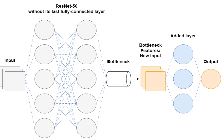
Since we already know the values being passed to our added layer, we can extract their values ahead of time by passing our inputs through ResNet-50 without its last full-connected layer. We can then use these features as our new input, essentially, bypassing all of ResNet-50's layers. Now, let's see how it performed.
Here, I've opted to use OrdinalEncoder instead of OneHotEncoder to save memory. If we had around 8000 observations/instances OneHotEncoder would create an 8000(# of observations/instance) x 133 (# classes) array, while OrdinalEncoder only creates an 8000 x 1 array.
Random state was set to 42 to keep the other bottleneck features' observation/incidents in the same order.
Here, we're compiling a model that accepts inputs that are the same shape as "resnet50_features" (bottleneck features). Refering back to figure 7, the function "model_top" is adding the "added layer."
You may have noticed that we didn't implement callback functions up until this point. For some reason, callbacks weren't working, but worry not! They're back and working. In this section we'll be making a function ( "callbacks_funcv2") to return the callbacks we want use—ModelCheckpoint, EarlyStopping, CSVLogger—and implement them in our training. For more information on callbacks, please refer to https://keras.io/api/callbacks/. Now, let's get to training
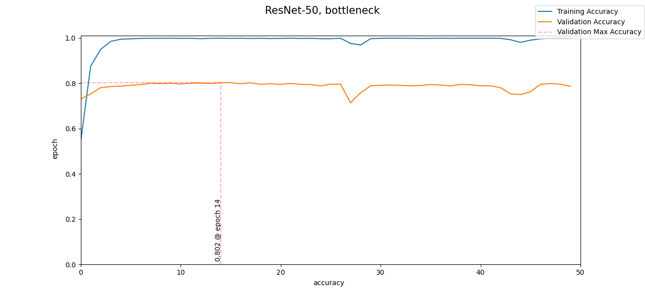
I was humbled after seeing these results. Before, every epoch took over an hour. With bottleneck features, 50 epochs took less than 2 minutes. Furthermore, it acheived 80% accuracy within 14 epochs (~36 seconds). This was far better than any efforts made by me in a span of [redacted] weeks. I would be lying if I said I wasn't embarrased or dismayed, however, I was equally amazed and hopeful in being able to reach 90% accuracy. Let's see what we can do with this new found knowledge.
In this section, we'll concoct a cocktail of concatenated convolution neural networks. Using the approach in section 4, we'll extract the bottleneck features of four neural networks and concat them into one dense layer. Then we'll add another dense layer just before the output layer. We'll be extracting the bottleneck features of the four, best-performing, midsized, neural networks: ResNet-152V2, Xception, Inception-ResNetV2, and EfficientNet-B7.
*as much as I would've liked to have used larger networks, due to memory constraints, I limited my choices to midsized networks
Here's a visual representation of what's going on.
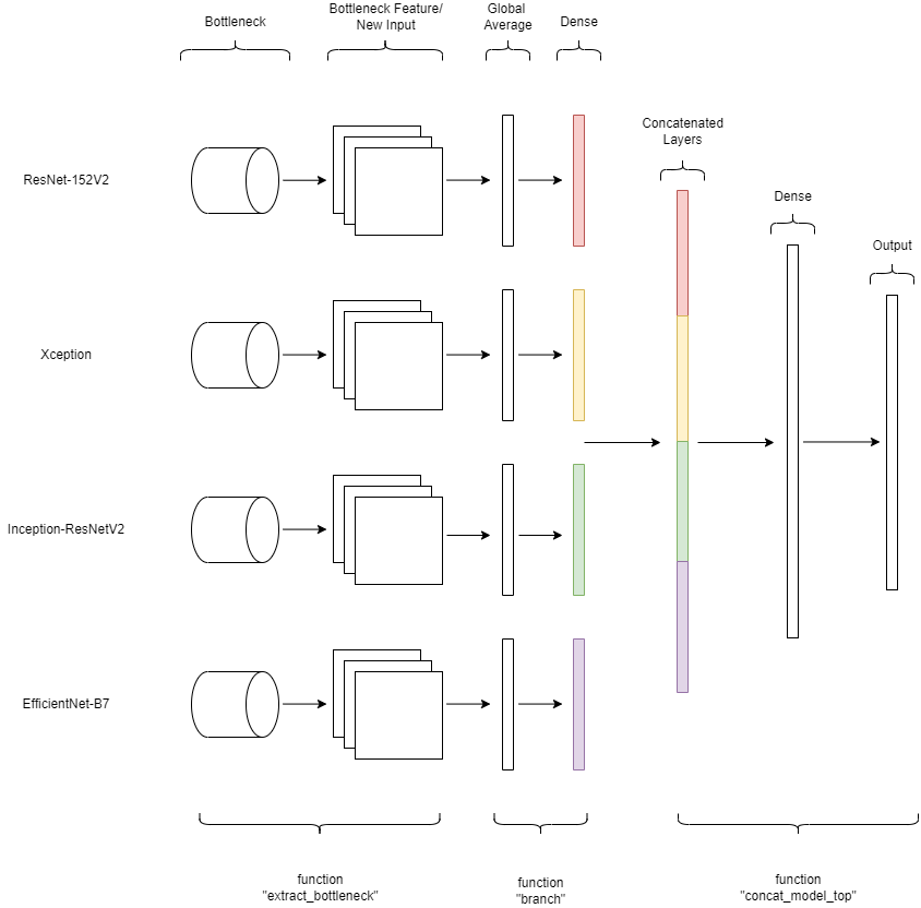
Let's take a look at the four best models. The four models being displayed below have been tuned by adjusting the "drop" and "reg" parameters in the functions "branch" and "concat_model_top."
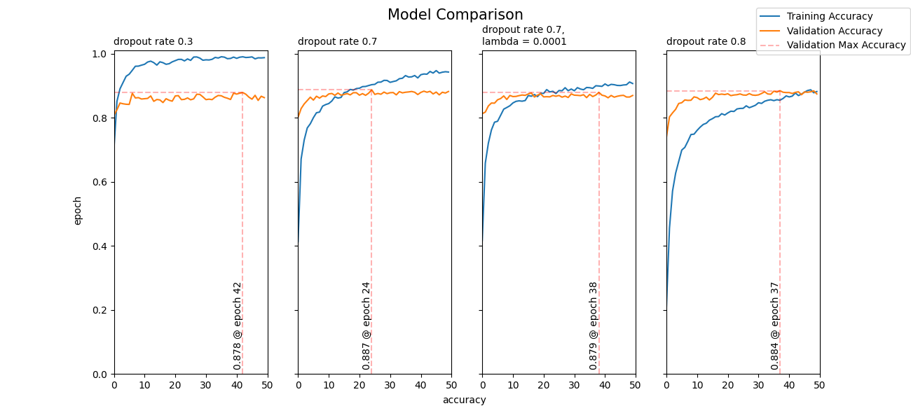
Stunning! After much training, I was able to get an accuracy of 89%. Although it's a percentage point less than 90%, I was satisfied with the results. Now, let's test our model on real world examples! We'll be using the second model with a dropout rate of 0.7, as it performed the best.
Before applying our model, we have some cleaning up to do. As of now, our model takes in four different bottleneck features as inputs, but we need it to take in one 200 by 200 by 3 image input. In order to do this, we need to reconstruct our model.
Now, that we have our complete model, let's get to applying!
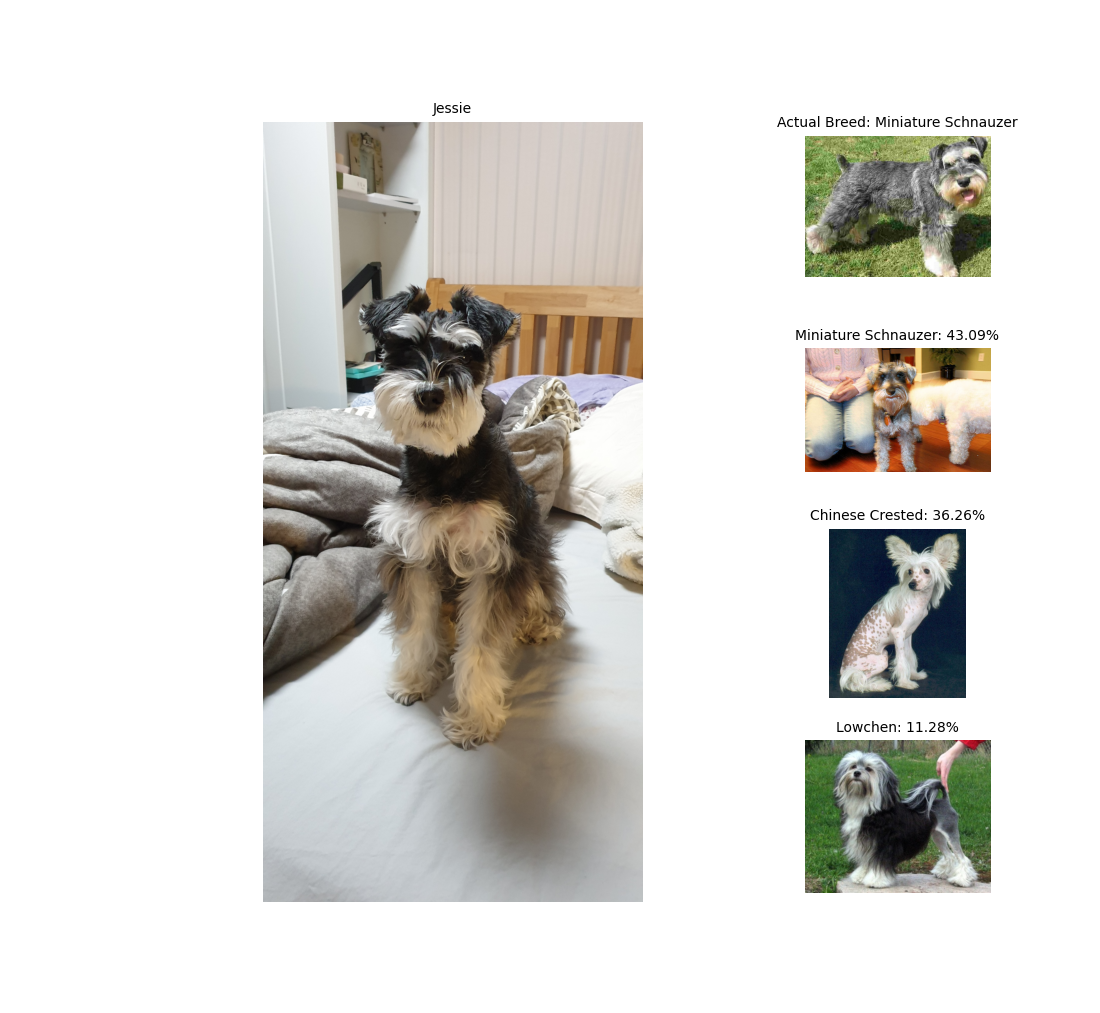
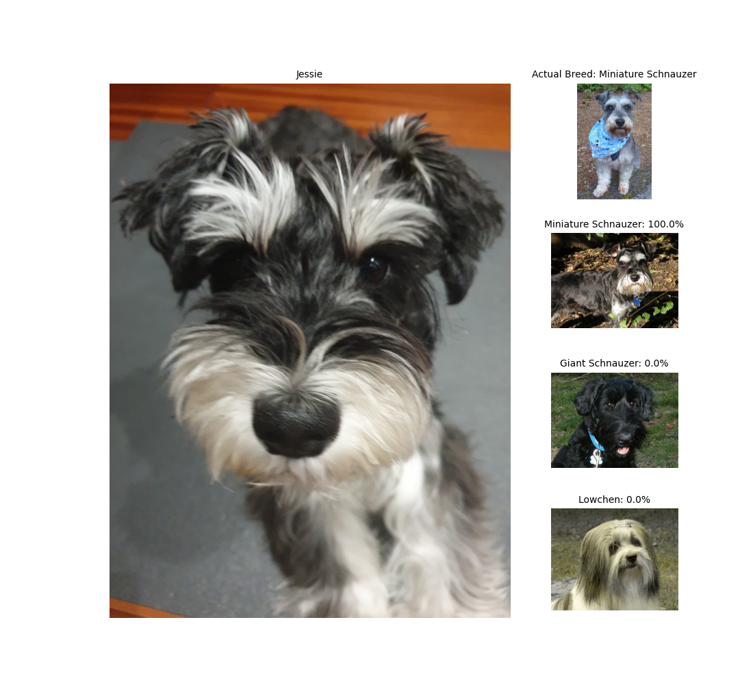
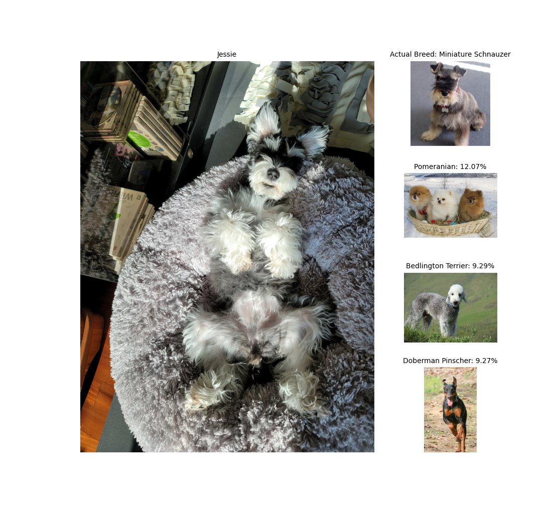
The functions used in this section are collapsed below. Also, please don't forget to give our friends below a little pet! You may or may not be pleasantly surprised.
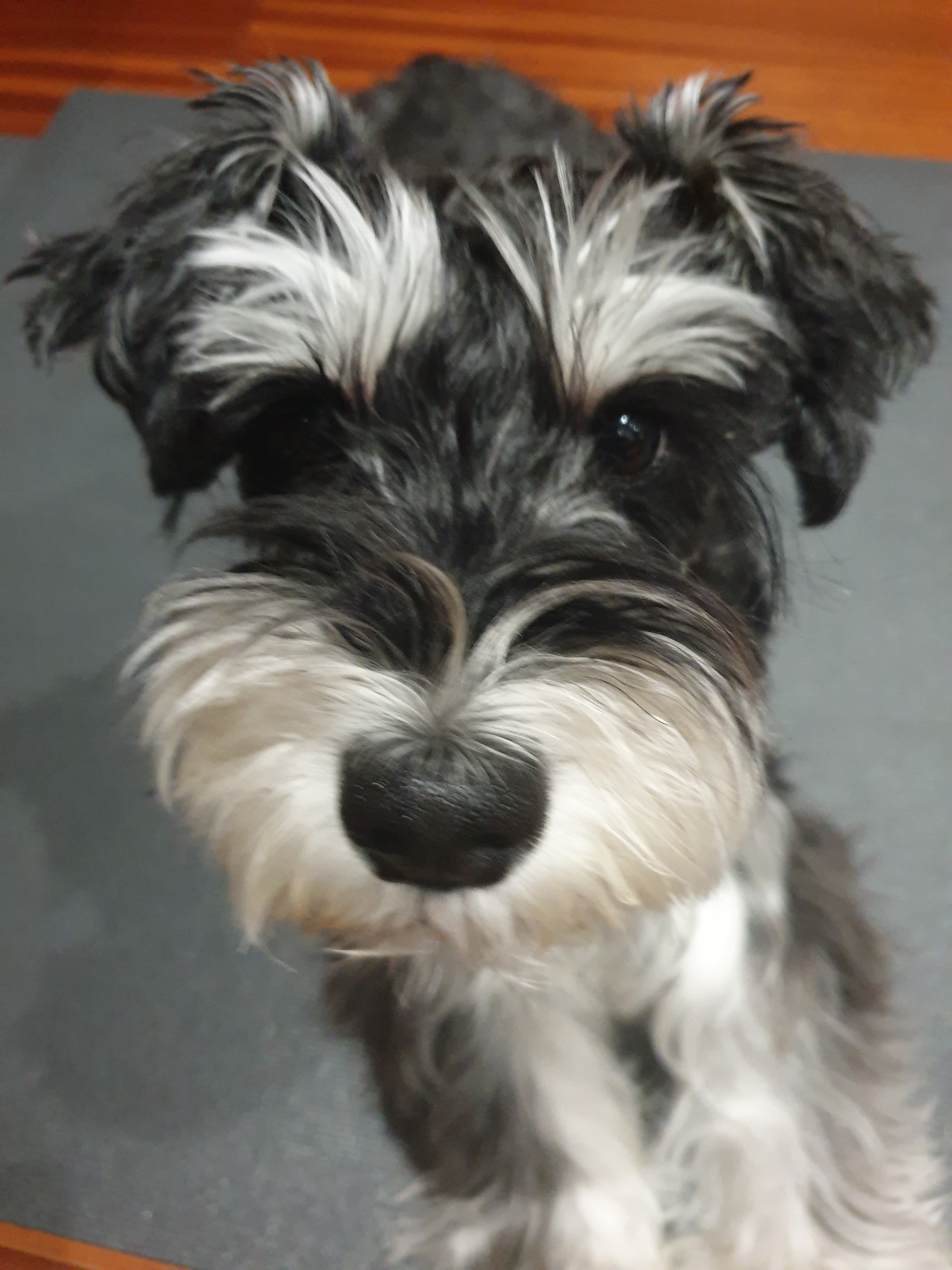
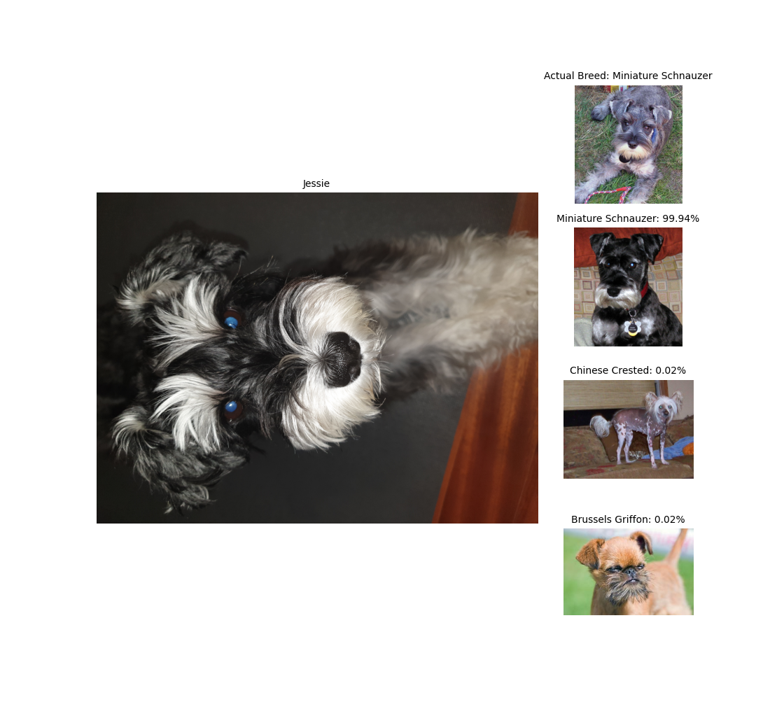
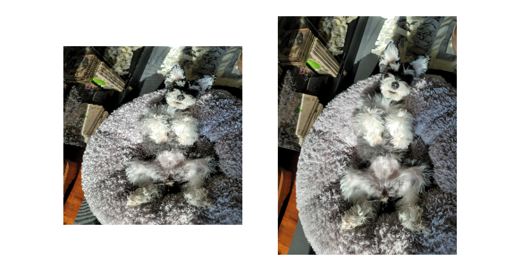
This is Jessie. She's a Miniature Schnauzer. We adopted her from the rescue center at the age of 3 to 4. Now, she's around 8 to 9 years young, and still gets mistaken as puppy! She's a very playful, yet gentle dog and she knows many, many tricks. Her favorite pastimes are sniffing around the house, playing fetch, and asking for scritches. Now, let's test our model on four different pictures of Jessie.
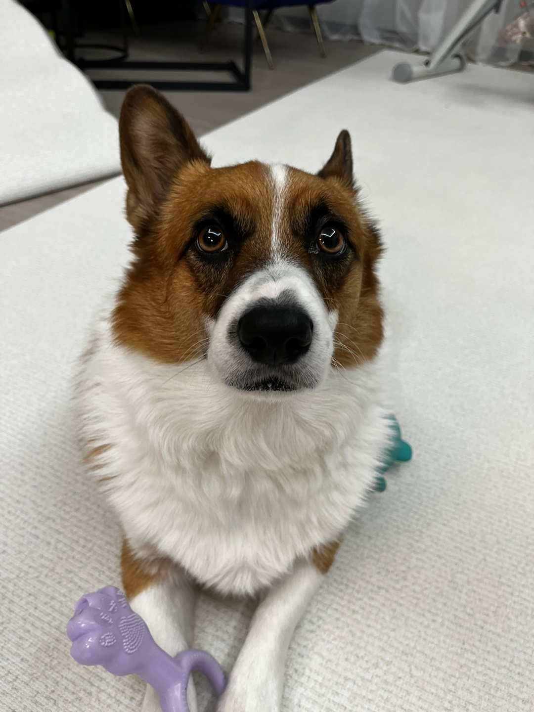
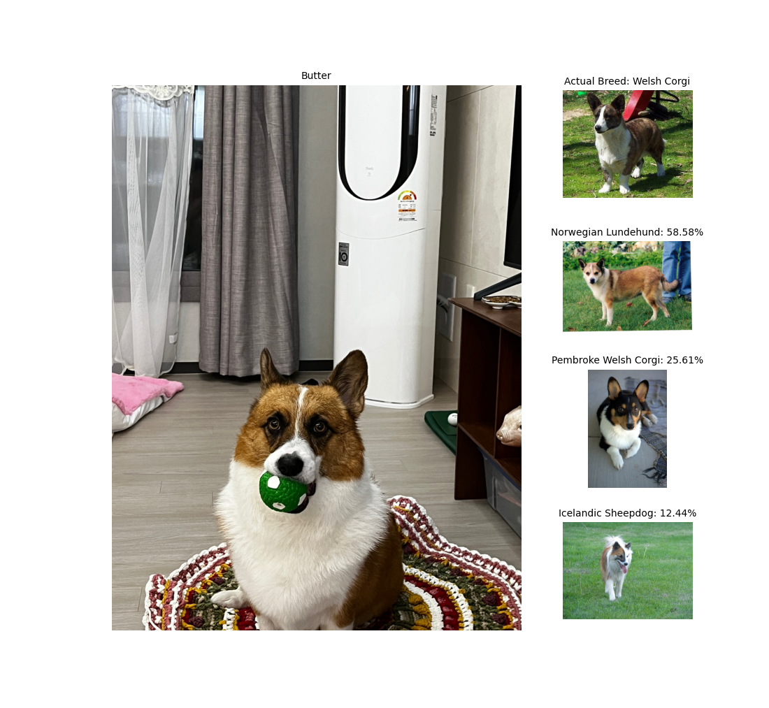
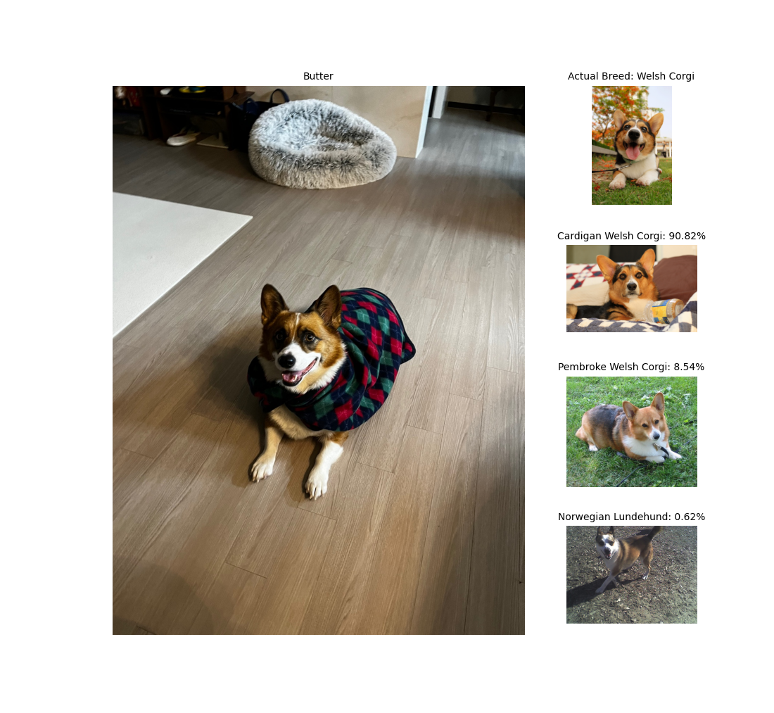
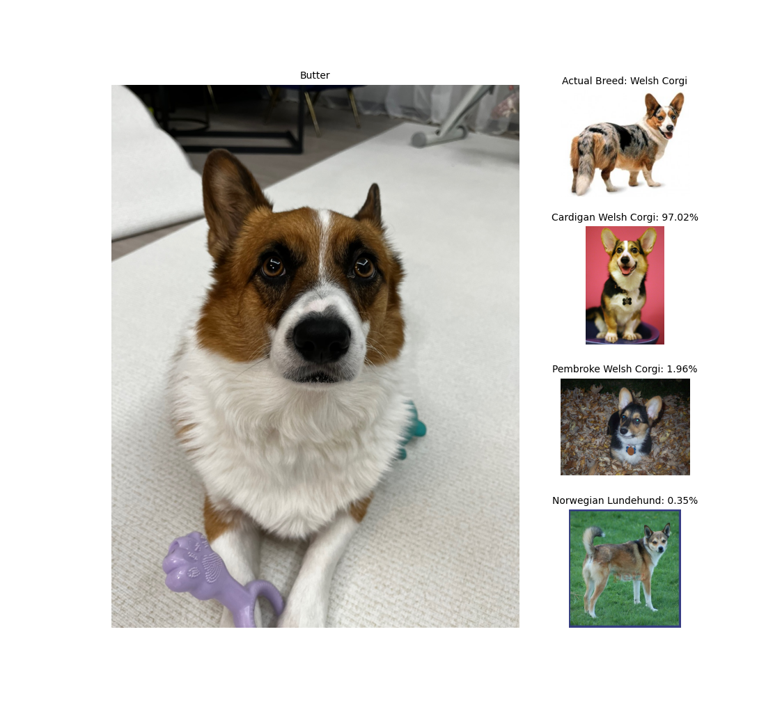
This is Butter. He's a 4 year old Welsh Corgi. He likes to bark at motorcycles and doesn't like Shibas. Now, let's test our model on three different pictures of Butter.
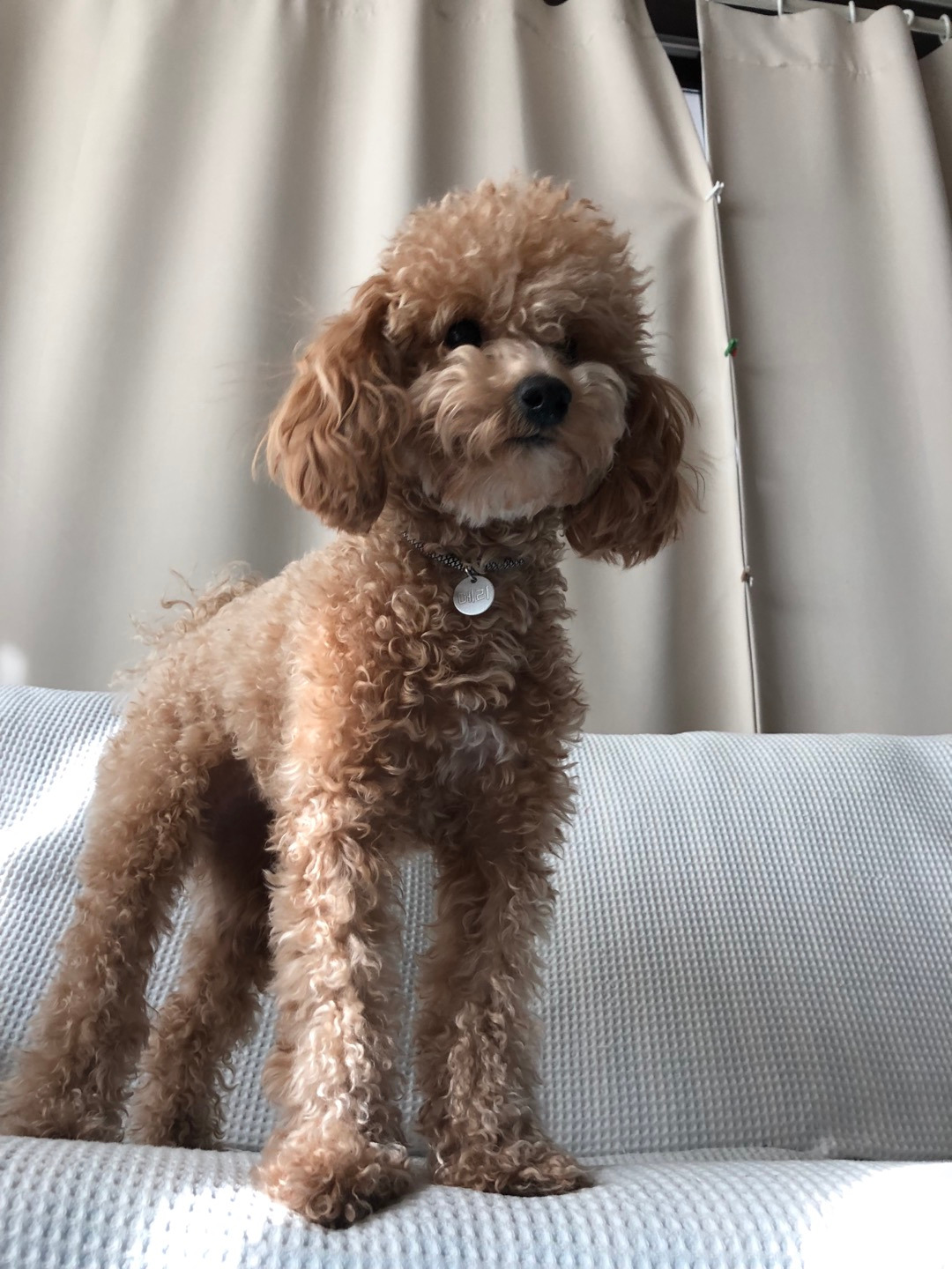
This is Merry, a 6 year old Minature Poodle. Her name is Merry because she was adopted on Christmas. She's a cute, sassy little lady that loves people and is afraid of the wind. Now, let's test our model on three different pictures of Merry.
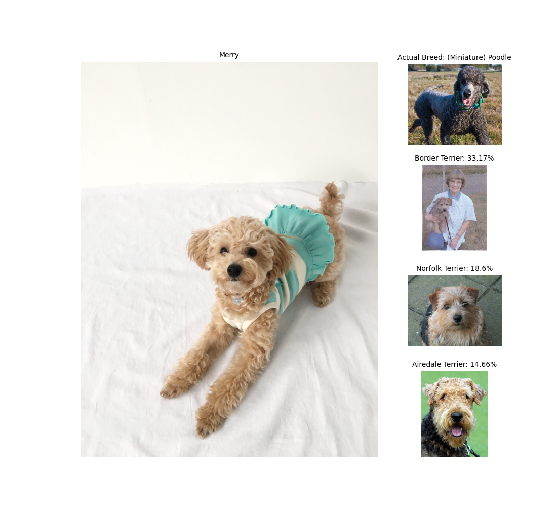
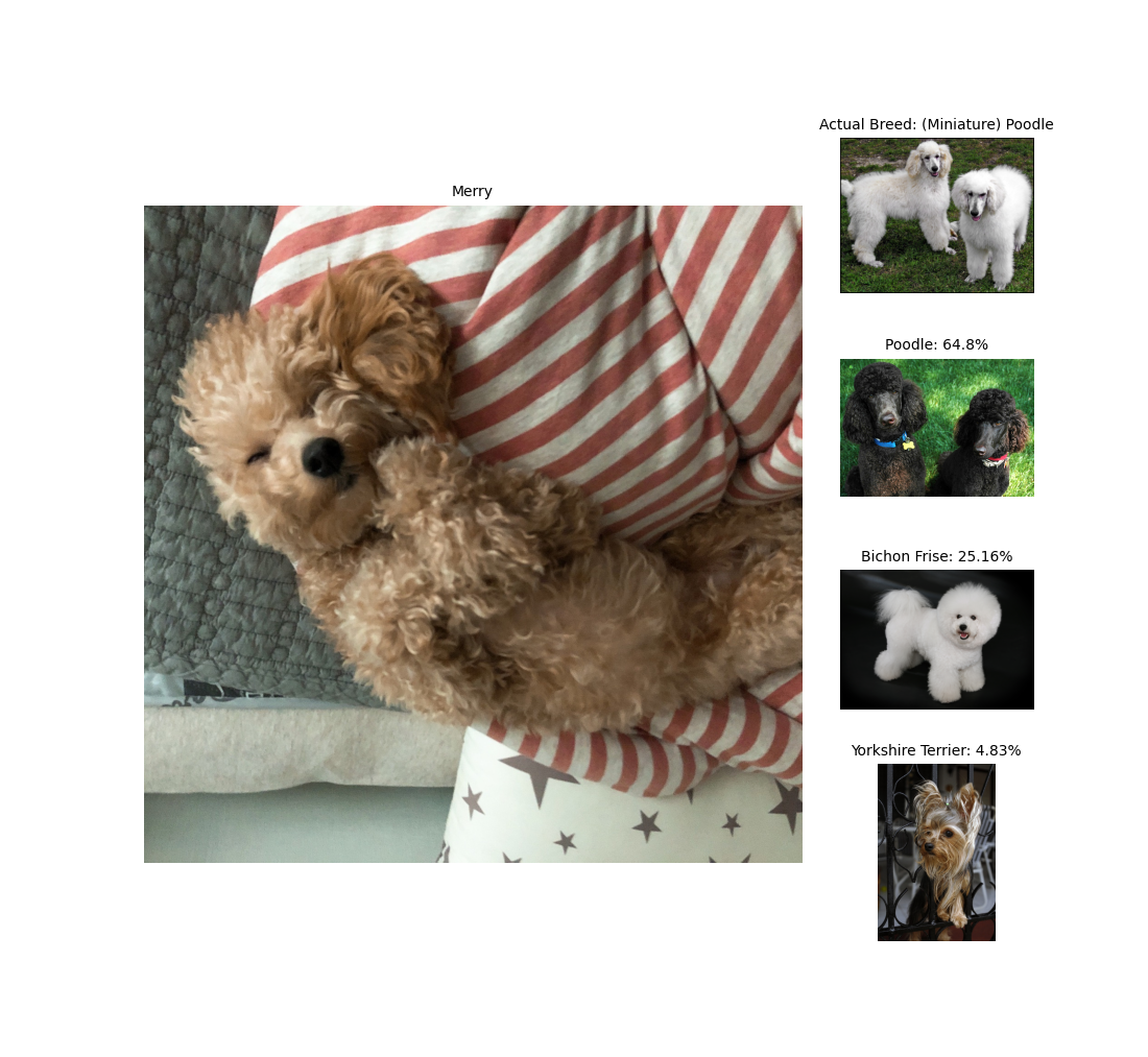
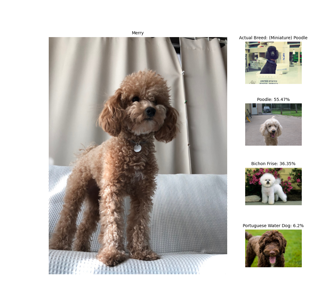
*the dataset I used to train the model did not differentiate Standard Poodles from Miniature Poodles
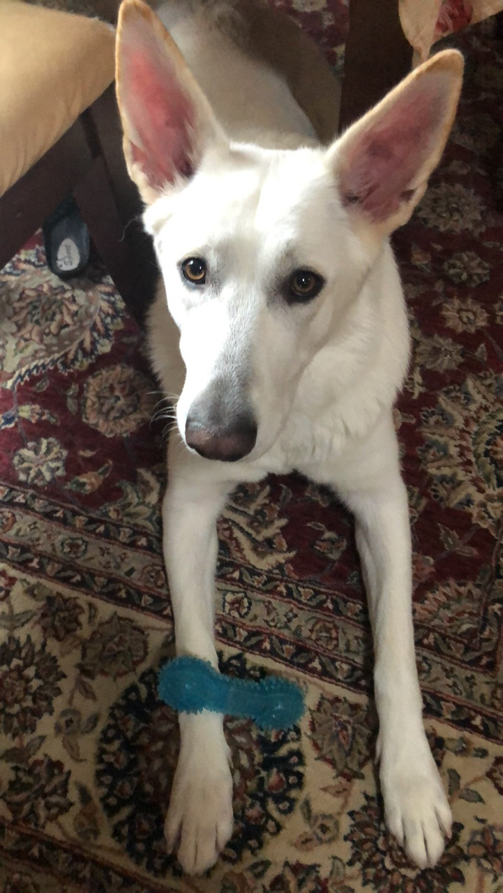
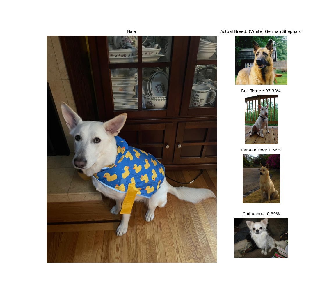
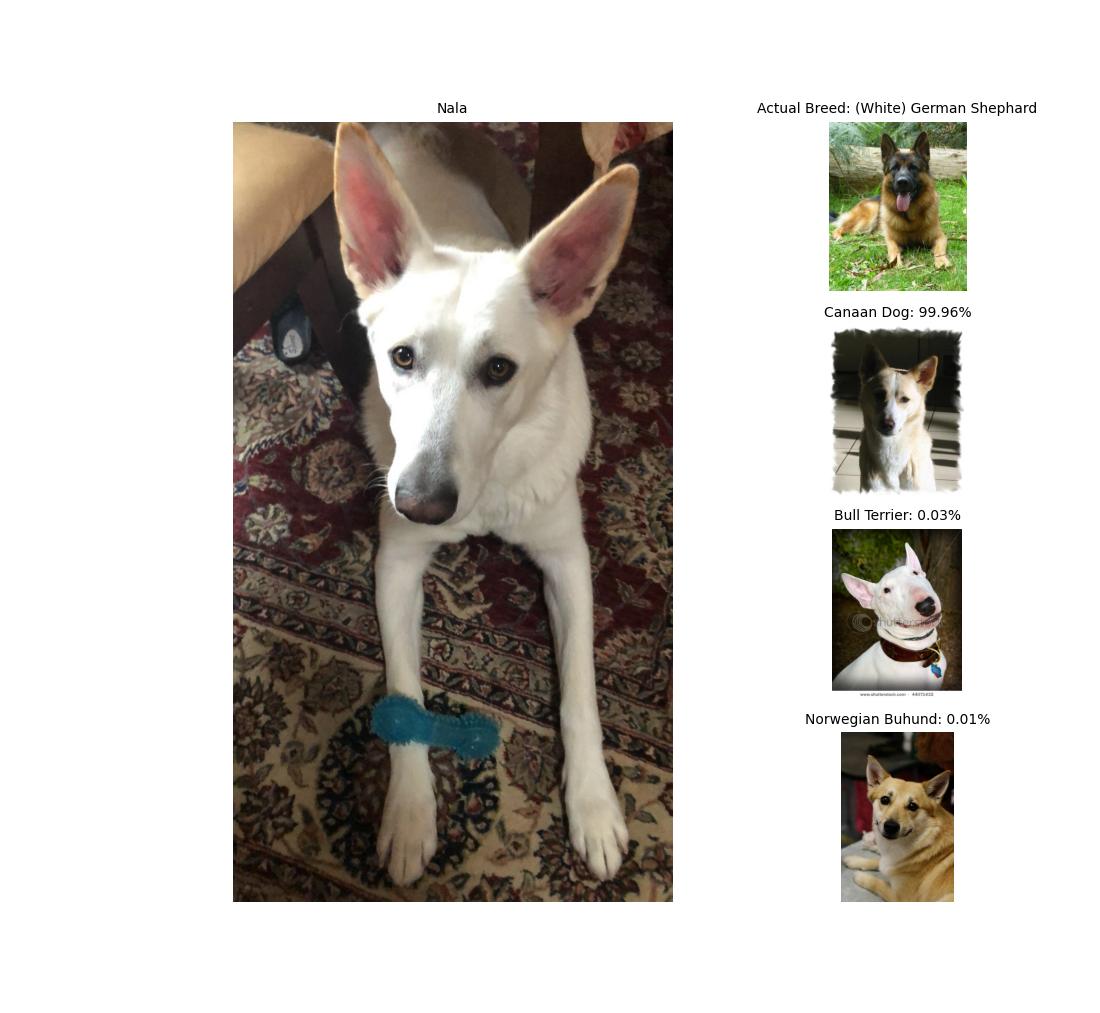
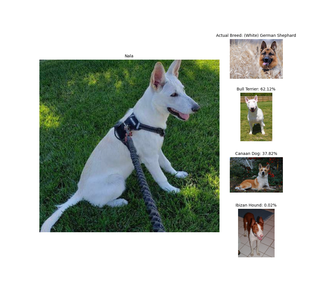
This is Nala. She's a 2 year old White German Shephard. She is named after the lioness in the movie, The Lion King. She loves to crawl underneath chairs and runs away from ear medicine. Now, let's test our model on three different pictures of Nala.
Overall, it was a difficult, but rewarding project. Getting to look at pictures of dogs was also a great stress-reliever. If I weren't constrained by my laptop's hardware, there are several things I would have done that would have drastically improved the accuracy of my model. For one, I would have combined larger networks. I could have also used the newly released Efficient Nets. Unfortunately, they weren't available when embarking on this project. I could have also used larger input images. During resizing, some images were affected more than others and a significant amount of noise was added to the pictures.
Lastly, another idea I had while searching for a better solution was to integrate a model like You Only Look Once (YOLO) to draw square anchor boxes around the dogs and extracting only the image inside the box. By limiting the anchor boxes to a square, we can resize the images into a standard size without skewing the proportions of a dog's features, which are probably pretty important for discerning a dog's breed. I would have loved to have pursued this idea if time permitted. Nonetheless, it's in my list of projects to complete. Be on the lookout!
If you'd like to know more about neural networks, please check out professor Andrew Ng's lectures on Youtube or Coursera. My ResNet-18 function was directly influenced by his assignments. Also, please check out the two links below. The idea to extract bottleneck features and concatenate them were inspired by a mixture of these two blog posts.
Thank you for reading! This page was generated entirely by me :) Please check out my GitHub repository to see the source code for this project as well as the source code for this page.